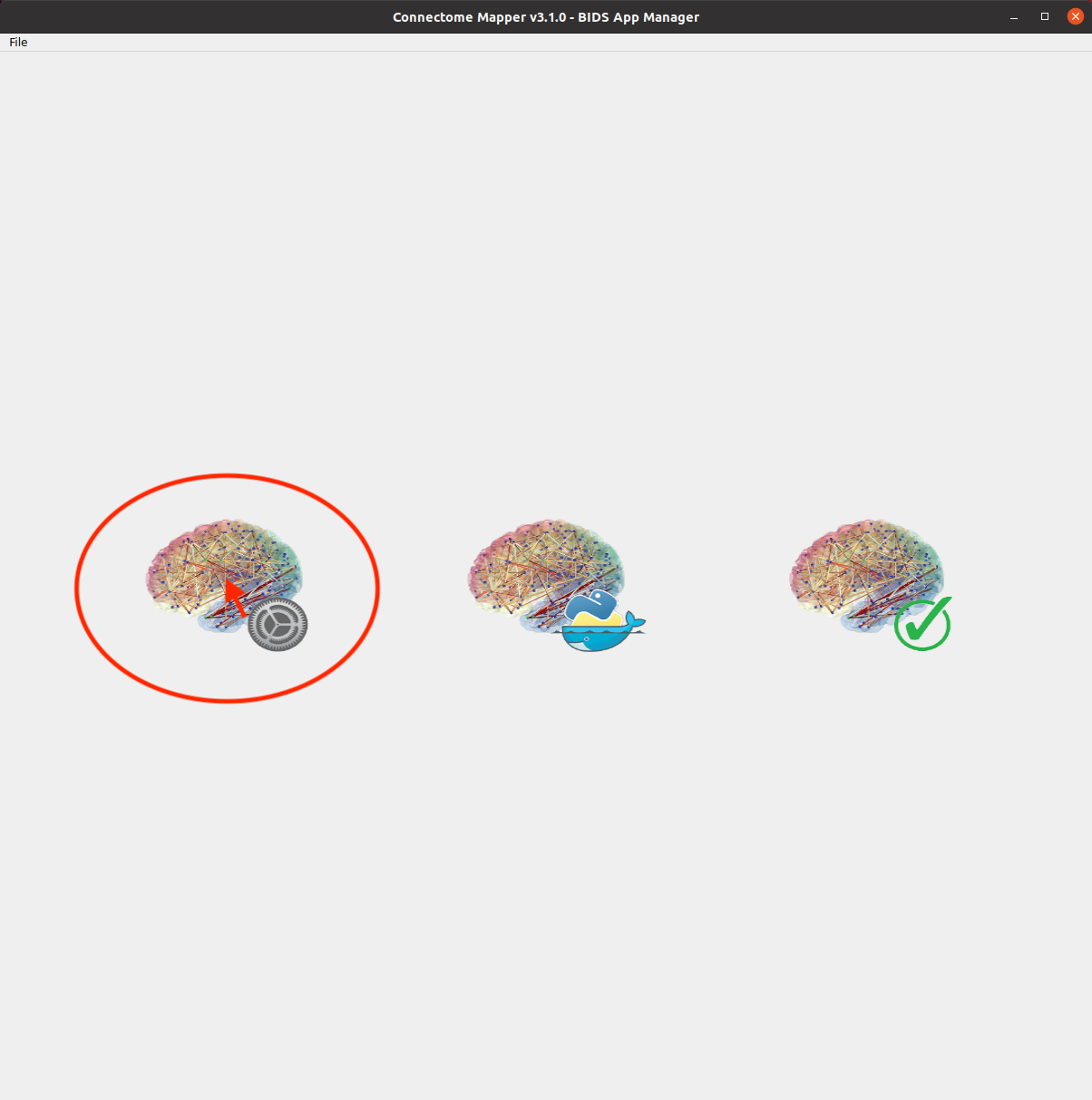
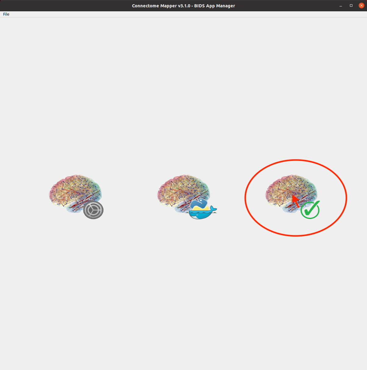
Connectome Mapper 3 comes with a Graphical User Interface, the Connectome Mapper BIDS App manager, designed to facilitate the configuration of all pipeline stages, the configuration of the BIDS App run and its execution, and the inspection of the different stage outputs with appropriate viewers.
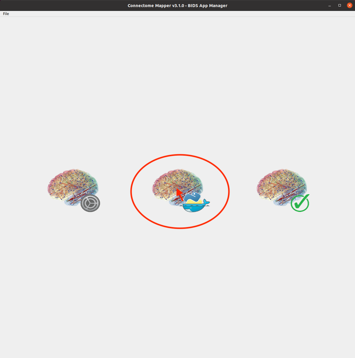
Main window of the Connectome Mapper BIDS App Manager
Click on File->LoadBIDSdataset... in the menu bar of the main window. Note that on Mac, Qt turns this menu bar into the native menu bar (top of the screen).
The ConnectomeMapper3 BIDS App Manager gives you two different options:
LoadBIDSdataset: load a BIDS dataset stored locally.
You only have to select the root directory of your valid BIDS dataset (see note below)
InstallDataladBIDSdataset: create a new datalad/BIDS dataset locally from an existing local or remote datalad/BIDS dataset (This is a feature under development)
If ssh connection is used, make sure to enable the “install via ssh” and to provide all connection details (IP address / Remote host name, remote user, remote password)
Note
The input dataset MUST be a valid BIDS structured dataset and must include at least one T1w or MPRAGE structural image. We highly recommend that you validate your dataset with the free, online BIDS Validator.
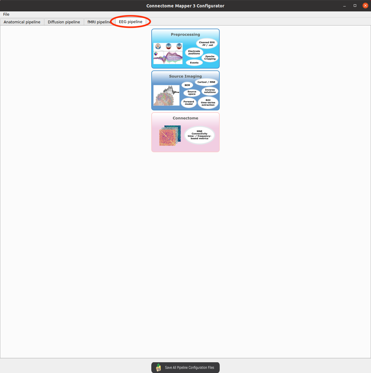
From the main window, click on the left button to start the Configurator Window.
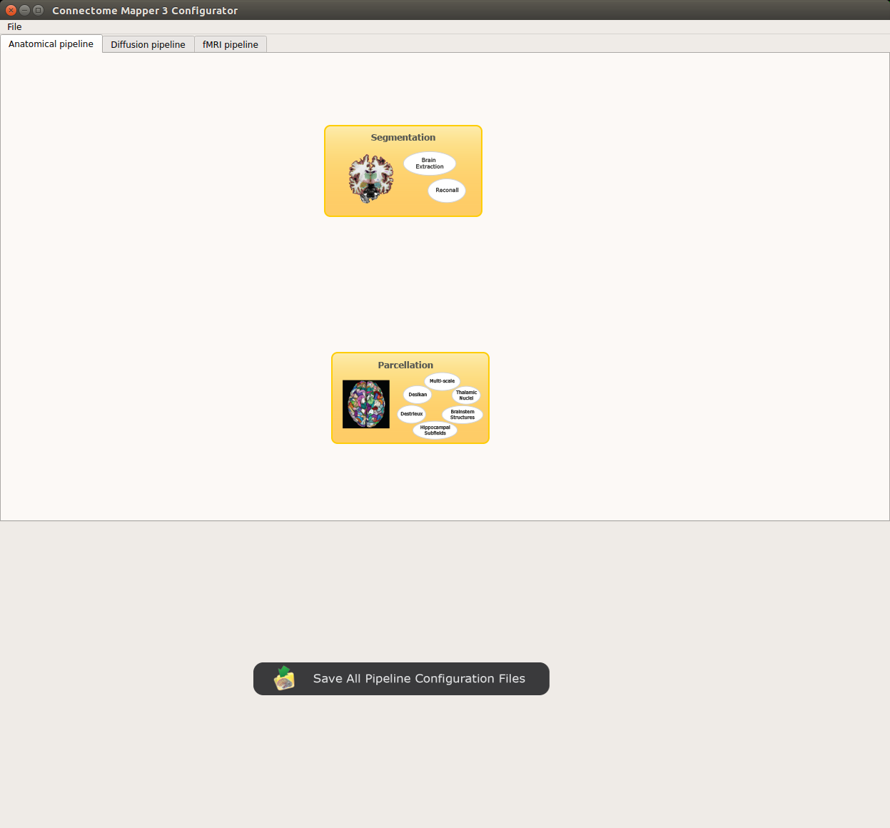
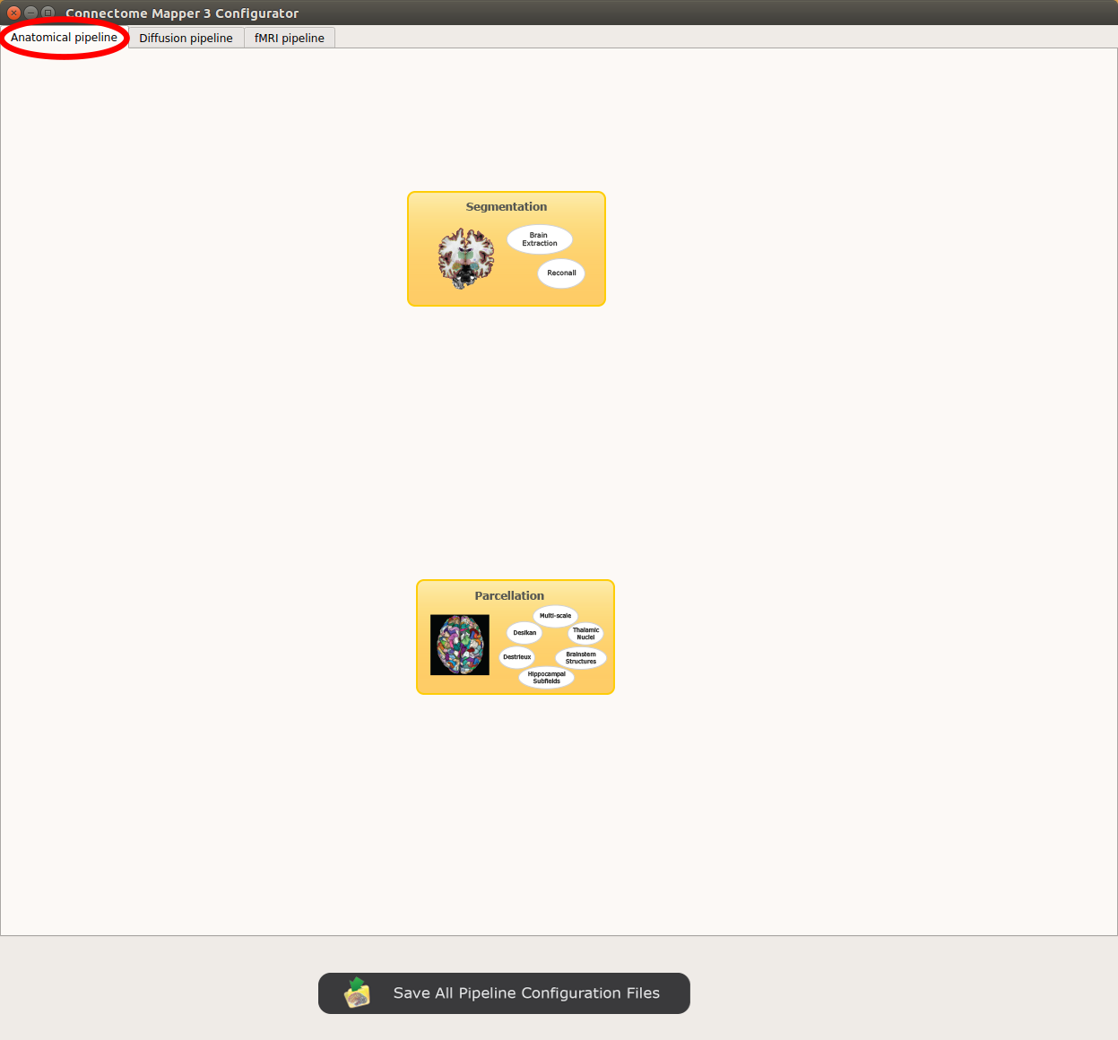
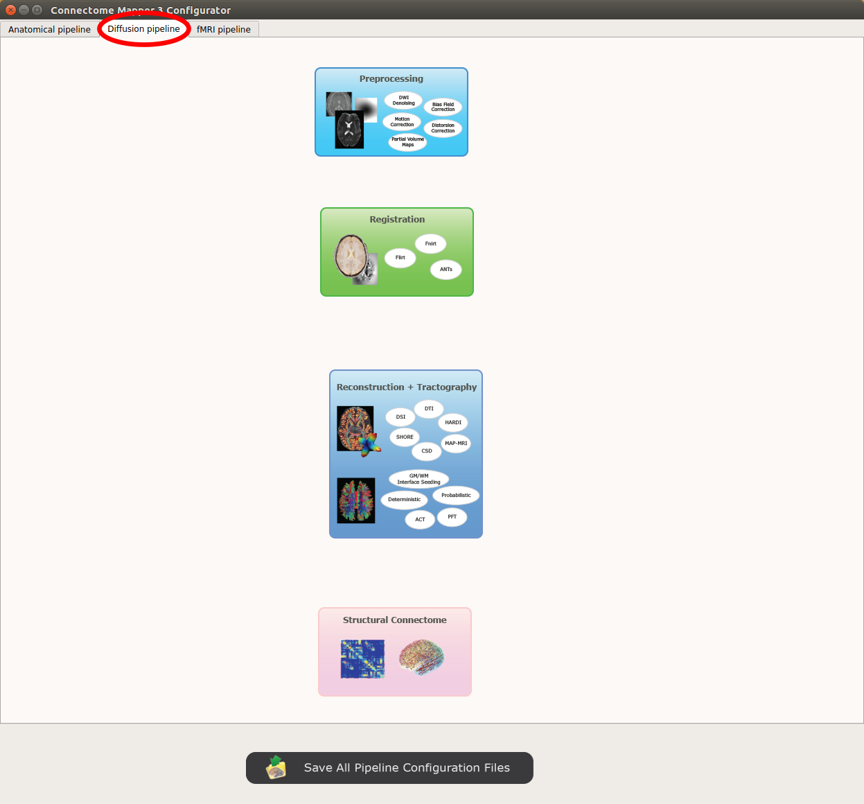
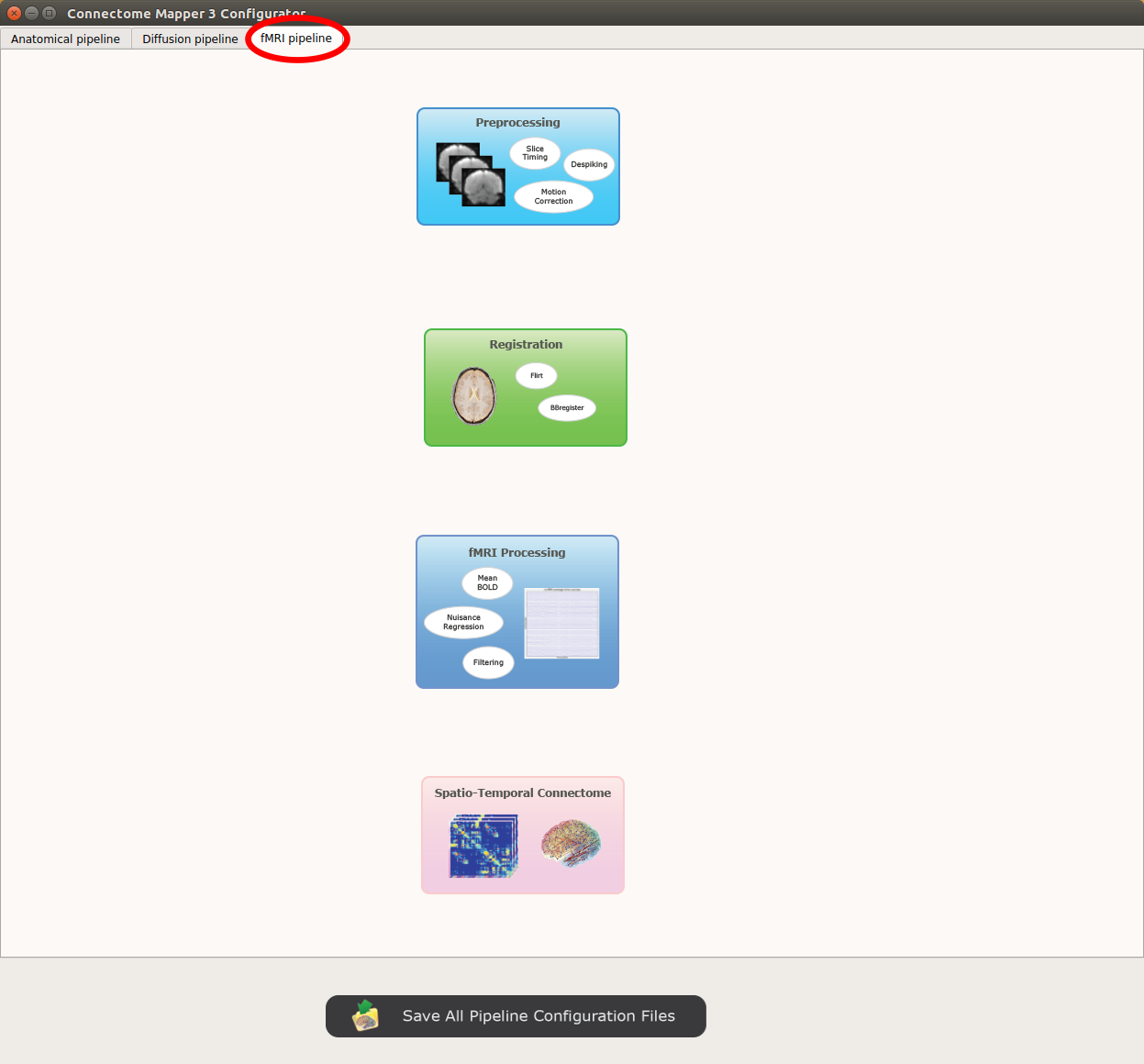
The window of the Connectome Mapper BIDS App Configurator will appear, which will assist you note only in configuring the pipeline stages (each pipeline has a tab panel), but also in creating appropriate configuration files which could be used outside the Graphical User Interface.
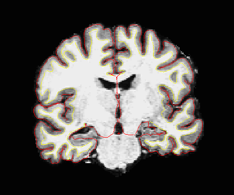
Prior to Lausanne parcellation, CMP3 relies on Freesurfer for the segmentation of the different brain tissues and the reconstruction of the cortical surfaces.
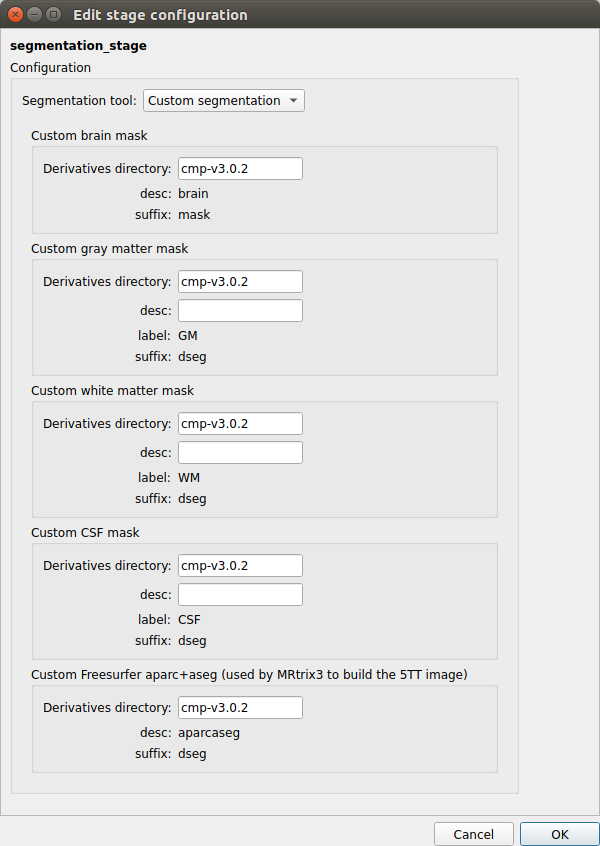
If you plan to use a custom parcellation, you will be required here to specify the pattern of the different existing segmentation files
that follows BIDS derivatives (See Custom segmentation).
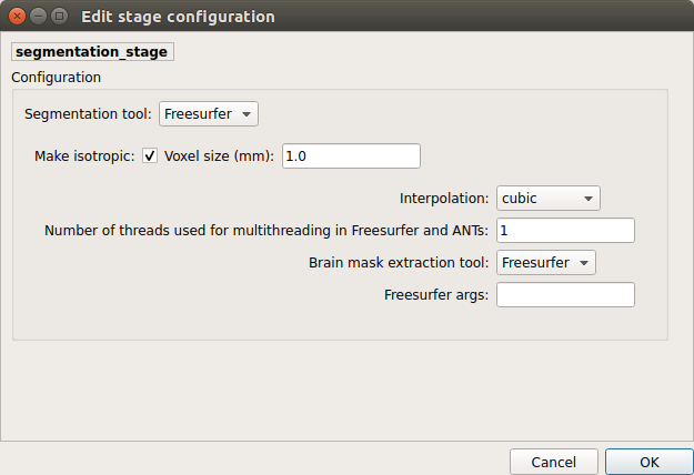
Freesurfer
Number of threads: used to specify how many threads are used for parallelization
Brain extraction tools: alternative brain extraction methods injected in Freesurfer
Freesurfer args: used to specify extra Freesurfer processing options
Note
If you have already Freesurfer v5 / v6 / v7 output data available, CMP3 can use them if there are placed in your output / derivatives directory.
Note however that since v3.0.3, CMP3 expects to find a freesurfer-7.1.1, so make sure that your derivatives are organized as
follows:
You can use any parcellation scheme of your choice as long as you provide a list of segmentation files organized following the BIDS derivatives specifications for segmentation files, provide appropriate .tsv sidecar files that describes the index/label/color mapping of the parcellation, and adopt the atlas-<label> entity to encode the name of the atlas, i.e:
The desc BIDS entity can be used to target specific mask and segmentation files.
For instance, the configuration above would allows us to re-use the outputs of the anatomical pipeline obtained with the previous v3.0.2 version of CMP3:
If you plan to use either Anatomically Constrained or Particle Filtering tractography, you will still require to have Freesurfer 7 output data available in your output / derivatives directory, as described the above note in *Freesurfer*.
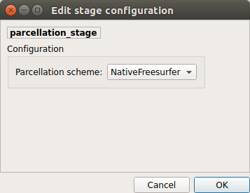
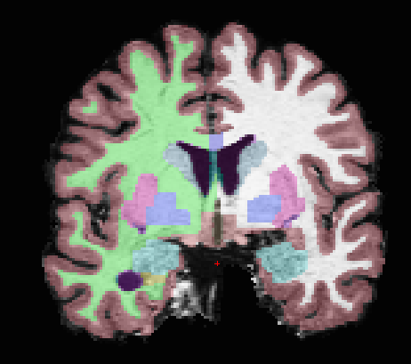
Generates the Native Freesurfer or Lausanne2018 parcellation from Freesurfer data. Alternatively, since v3.0.3 you can use your own custom parcellation files.
Parcellation scheme
NativeFreesurfer:
Atlas composed of 83 regions from the Freesurfer aparc+aseg file
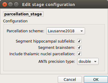
Lausanne2018:
New version of Lausanne parcellation atlas, corrected, and extended with 7 thalamic nuclei, 12 hippocampal subfields, and 4 brainstem sub-structure per hemisphere
Since v3.0.0, Lausanne2018 parcellation has completely replaced the old Lausanne2008 parcellation.
As it provides improvements in the way Lausanne parcellation label are generated,
any code and data related to Lausanne2008 has been removed. If you still wish to
use this old parcellation scheme, please use v3.0.0-RC4 which is the last version
that supports it.
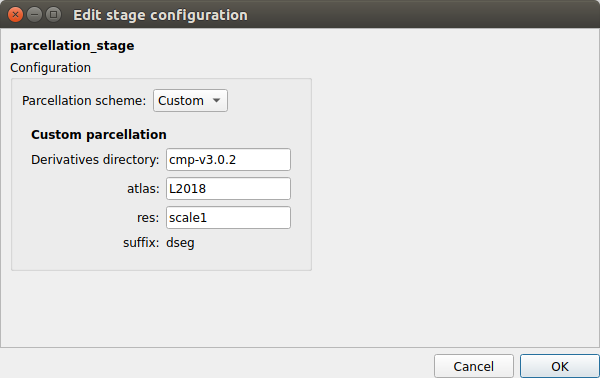
Custom:
You can use any parcellation scheme of your choice as long as they follow the BIDS derivatives specifications for segmentation files, provide appropriate .tsv sidecar files that describes the index/label/color mapping of the parcellation, and adopt the atlas-<label> entity to encode the name of the atlas, i.e:
The res BIDS entity allows the differentiation between multiple scales of the same atlas.
For instance, the above configuration would allows us to re-use the scale 1 of the Lausanne parcellation generated by the anatomical pipeline obtained of the previous v3.0.2 version of CMP3:
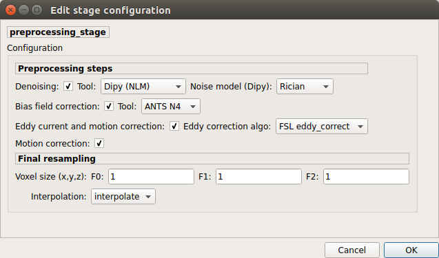
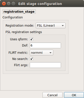
Preprocessing includes denoising, bias field correction, motion and eddy current correction for diffusion data.
Denoising
Remove noise from diffusion images using (1) MRtrix3 MP-PCA method or (2) Dipy Non-Local Mean (NLM) denoising with Gaussian or Rician noise models
Bias field correction
Remove intensity inhomogeneities due to the magnetic resonance bias field using (1) MRtrix3 N4 bias field correction or (2) the bias field correction provided by FSL FAST
Motion correction
Aligns diffusion volumes to the b0 volume using FSL’s MCFLIRT
Eddy current correction
Corrects for eddy current distortions using FSL’s Eddy correct tool
Resampling
Resample morphological and diffusion data to F0 x F1 x F2 mm^3
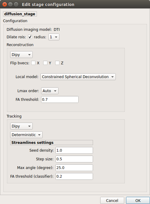
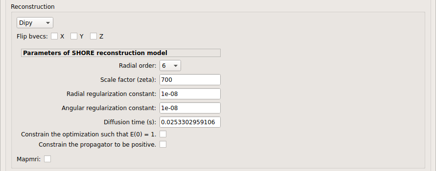
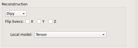
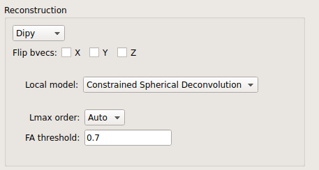
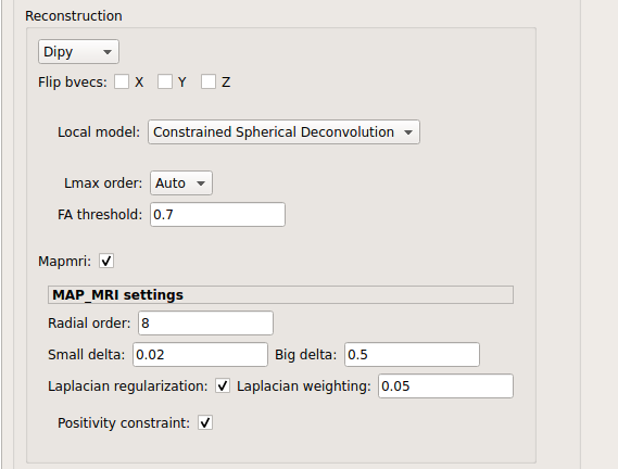
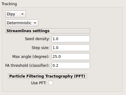
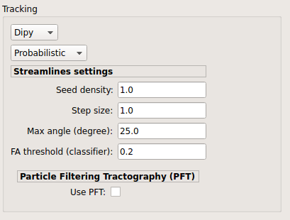
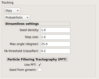
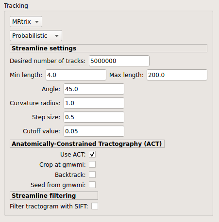
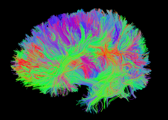
Perform diffusion reconstruction and local deterministic or probabilistic tractography based on several tools. ROI dilation is required to map brain connections when the tracking only operates in the white matter.
Probabilistic PFT tracking performed on SHORE or CSD reconstruction. Seeding from the gray matter / white matter interface is possible.
Note
We noticed a shift of the center of tractograms obtained by dipy. As a result, tractograms visualized in TrackVis are not commonly centered despite the fact that the tractogram and the ROIs are properly aligned.
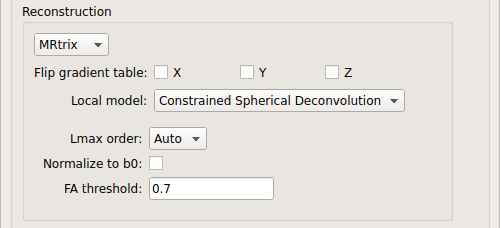
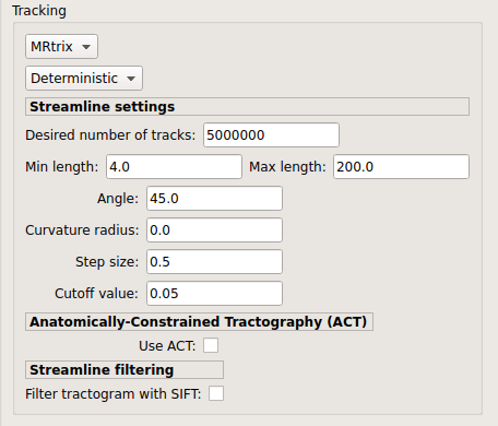
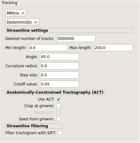
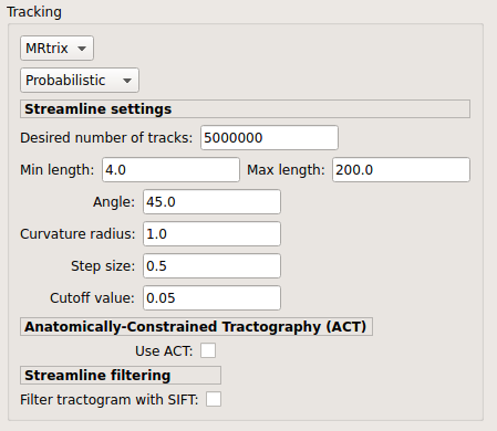
MRtrix: perform deterministic and probabilistic fiber tracking as well as anatomically-constrained tractography. ROI dilation is required to map brain connections when the tracking only operates in the white matter.
Deterministic tractography:
Deterministic tractography (SD_STREAM) performed on single tensor or CSD reconstruction
Deterministic ACT tracking performed on single tensor or CSD reconstruction. Seeding from the gray matter / white matter interface is possible. Backtrack option is not available in deterministic tracking.
Probabilistic tractography:
Probabilistic tractography (iFOD2) performed on SHORE or CSD reconstruction
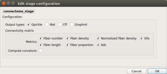
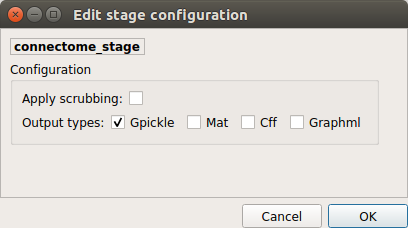
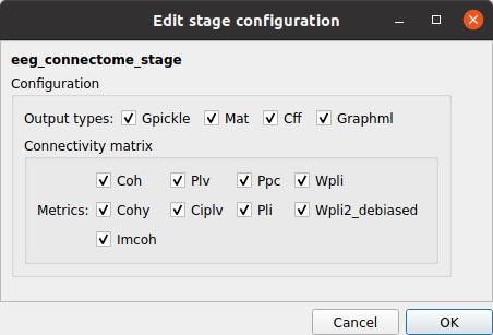
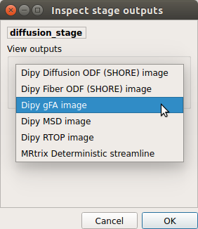
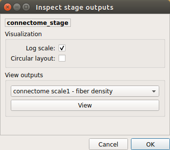
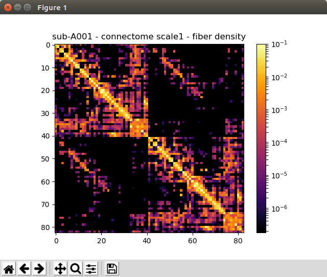
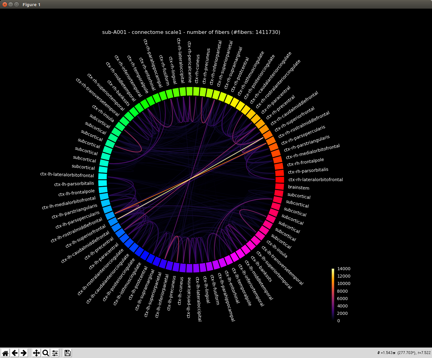
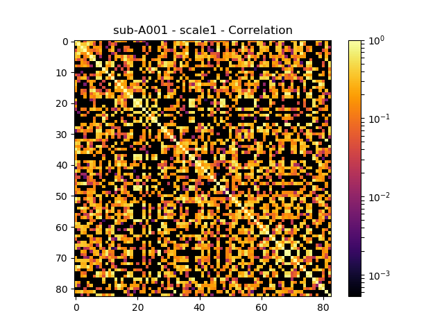
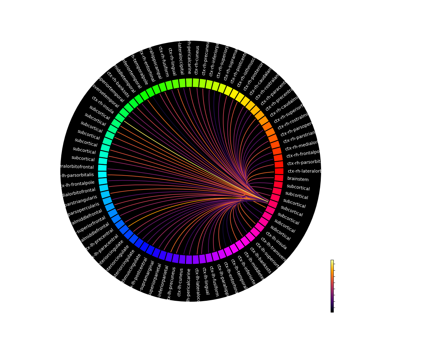
Compute fiber length connectivity matrices. If DTI data is processed, FA additional map is computed. In case of DSI, additional maps include GFA and RTOP. In case of MAP-MRI, additional maps are RTPP, RTOP, …
Output types
Select in which formats the connectivity matrices should be saved.
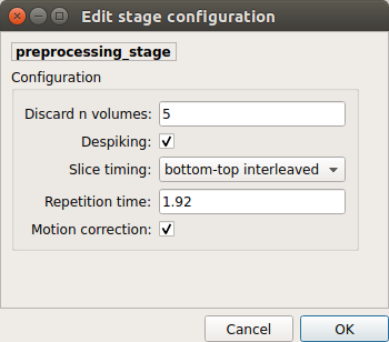
Preprocessing refers to processing steps prior to registration. It includes discarding volumes, despiking, slice timing correction and motion correction for fMRI (BOLD) data.
Discard n volummes
Discard n volumes from further analysis
Despiking
Perform despiking of the BOLD signal using AFNI.
Slice timing and Repetition time
Perform slice timing correction using FSL’s slicetimer.
Motion correction
Align BOLD volumes to the mean BOLD volume using FSL’s MCFLIRT.
Performs detrending, nuisance regression, bandpass filteringdiffusion reconstruction and local deterministic or probabilistic tractography based on several tools. ROI dilation is required to map brain connections when the tracking only operates in the white matter.
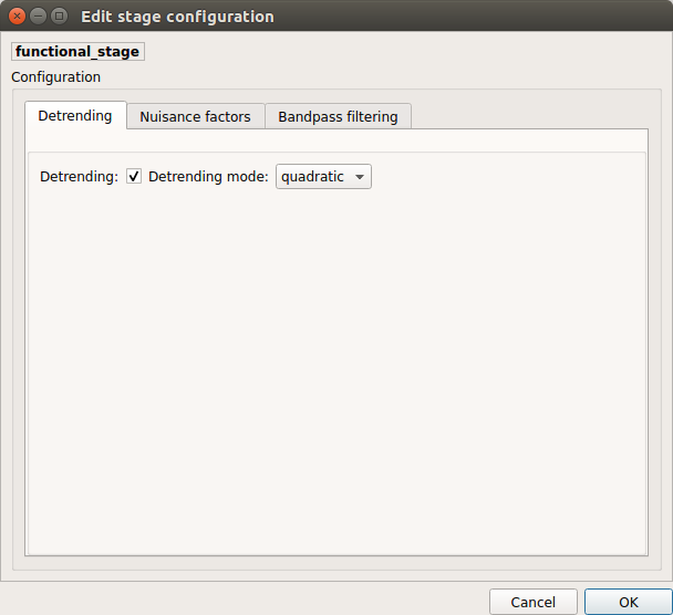
Detrending
Detrending of BOLD signal using:
linear trend removal algorithm provided by the scipy library
quadratic trend removal algorithm provided by the obspy library
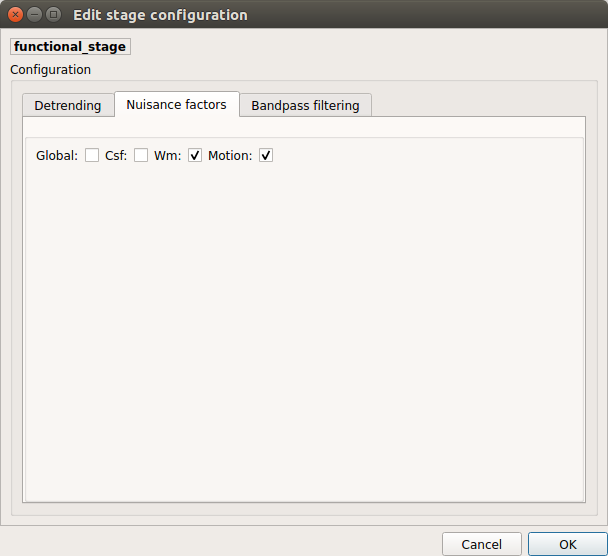
Nuisance regression
A number of options for removing nuisance signals is provided. They consist of:
Global signal regression
CSF regression
WM regression
Motion parameters regression
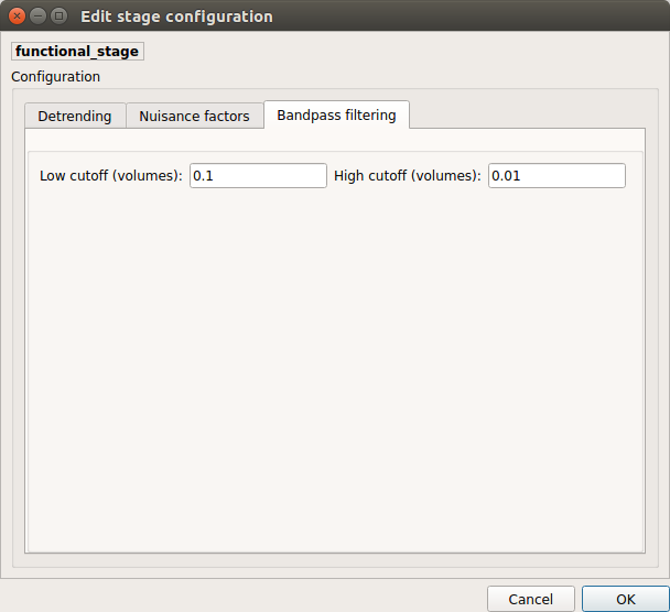
Bandpass filtering
Perform bandpass filtering of the time-series using FSL’s slicetimer
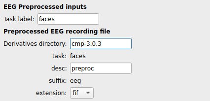
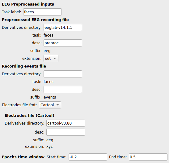
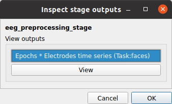
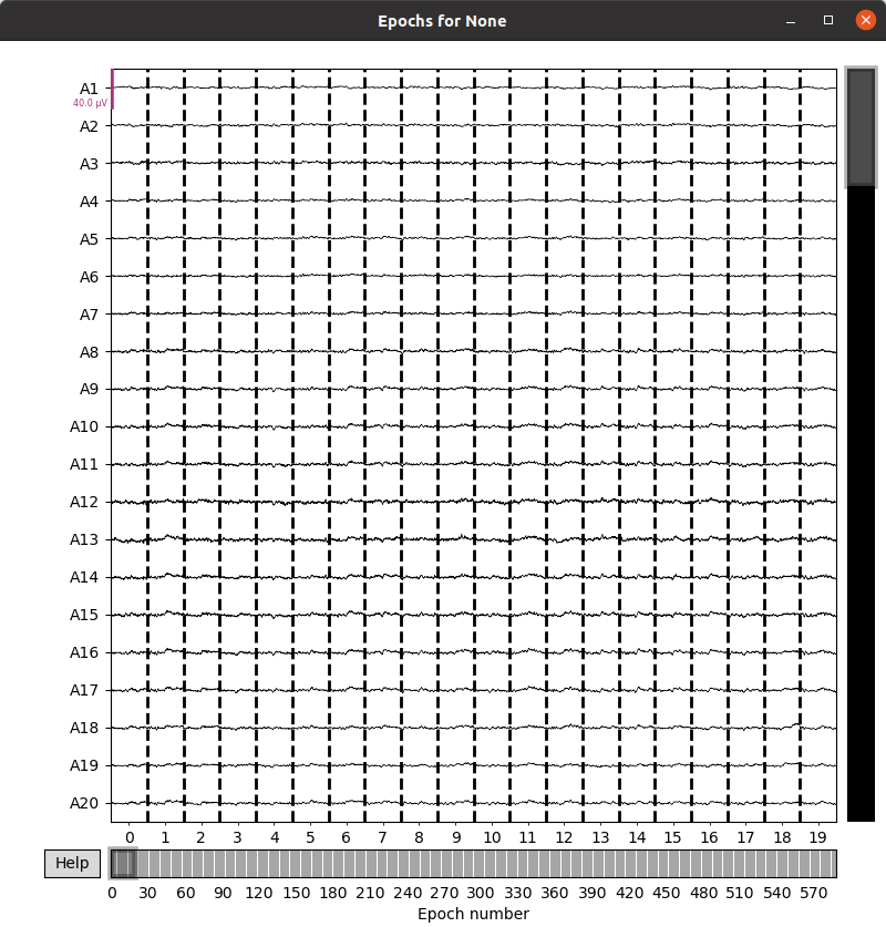
EEG Preprocessing refers to steps that loads, crop, and save preprocessed EEG epochs data of a given task in fif format, the harmonized format used further in the pipeline.
EEG data can be provided as:
A mne.Epochs object already saved in fif format:
A set of the following files and parameters:
Preprocessed EEG recording: store the Epochs * Electrodes dipole time-series in eeglab set format
Recording events file in BIDS *_events.tsv format: describe timing and other properties of events recorded during the task
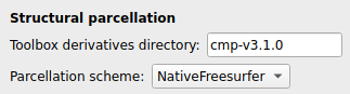
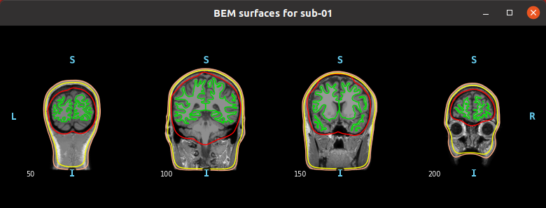
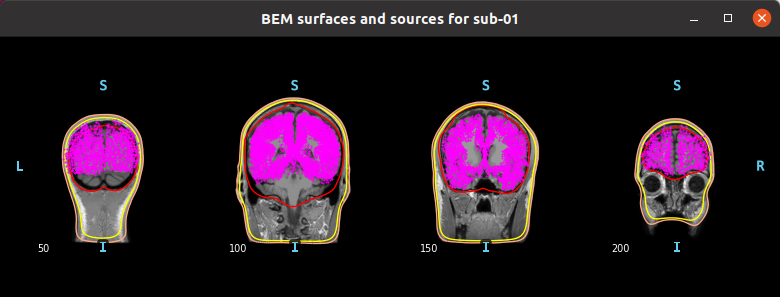
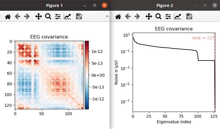
EEG Source Imaging refers to the all the steps necessary to obtain the inverse solutions and extract ROI time-series for a given parcellation scheme.
Structural parcellation: specify the cmp derivatives directory, the parcellation scheme, and the scale (for Lausanne 2018) to retrieve the parcellation files
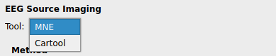
Tool: CMP3 can either leverage MNE to compute the inverse solutions or take inverse solutions already pre-computed with Cartool as input.
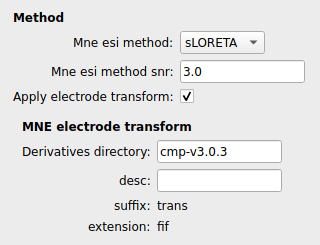
MNE
If MNE is selected, all steps necessary to reconstruct the inverse solutions are performed by leveraging MNE. In this case, the following files and parameters need to be provided:
MNE ESI method: Method to compute the inverse solutions
MNE ESI method SNR: SNR level used to regularize the inverse solutions
MNE electrode transform: Additional transform in MNE trans.fif format to be applied to electrode coordinates when Apply electrode transform is enabled
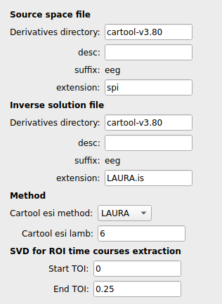
Cartool
If Cartool is selected, the following files (generated by this tool) and parameters need to be provided:
Source space file: *.spi text file with 3D-coordinates (x, y and z-dimension) with possible solution points necessary to obtain the sources or generators of ERPs
Inverse solution file: *.is binary file that includes number of electrodes and solution points
Cartool esi method: Method used to compute the inverse solutions (Cartool esi method)
Cartool esi lamb: Regularization level of inverse solutions
SVD for ROI time-courses extraction: Start and end TOI parameters for the SVD algorithm that extract single ROI time-series from dipoles.
You can save the pipeline stage configuration files in two different way:
You can save all configuration files at once by clicking on the SaveAllPipelineConfigurationFiles. This will save automatically the configuration file of the anatomical / diffusion / fMRI pipeline to
<bids_dataset>/code/ref_anatomical_config.ini / <bids_dataset>/code/ref_diffusion_config.ini / <bids_dataset>/code/ref_fMRI_config.ini, <bids_dataset>/code/ref_EEG_config.ini respectively.
You can save individually each of the pipeline configuration files and edit its filename in the File menu (File -> Save anatomical/diffusion/fMRI/EEG configuration file as…)
Connectome Mapper relies on Nipype.
All intermediate steps for the processing are saved in the corresponding
<bids_dataset/derivatives>/nipype/sub-<participant_label>/<pipeline_name>/<stage_name>
stage folder (See Nipype workflow outputs for more details).
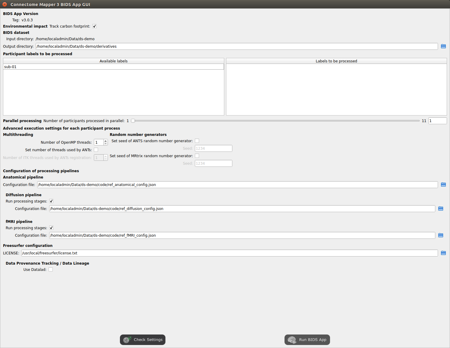
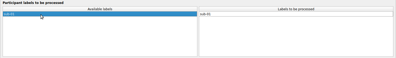
Tune the number of subjects to be processed in parallel
Tune the advanced execution settings for each subject process. This include finer control on the number of threads used by each process as well as on the seed value of ANTs and MRtrix random number generators.
Important
Make sure the number of threads multiplied by the number of subjects being processed in parallel do not exceed the number of CPUs available on your system.
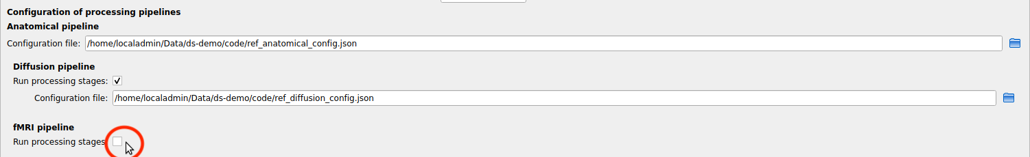
Check/Uncheck the pipelines to be performed
Note
The list of pipelines might vary as it is automatically updated based on the availability of raw diffusion MRI, resting-state fMRI, and preprocessed EEG data.
Specify your Freesurfer license
Note
Your Freesurfer license will be copied to your dataset directory as <bids_dataset>/code/license.txt which will be mounted inside the BIDS App container image.
When the run is set up, you can click on the Checksettings button.
If the setup is complete and valid, this will enable the RunBIDSApp button.
For each subject, the execution output of the pipelines are redirected to a log file, written as <bids_dataset/derivatives>/cmp-v3.X.Y/sub-<subject_label>_log.txt. Execution progress can be checked by the means of these log files.
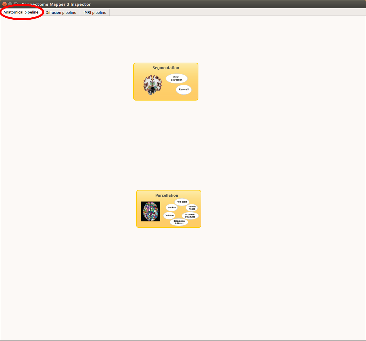
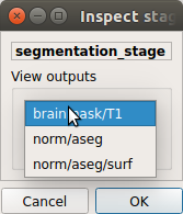
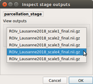
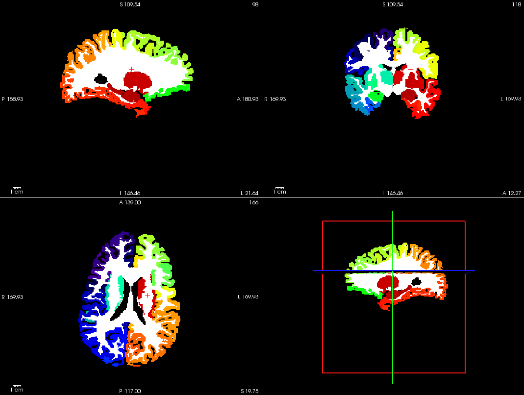
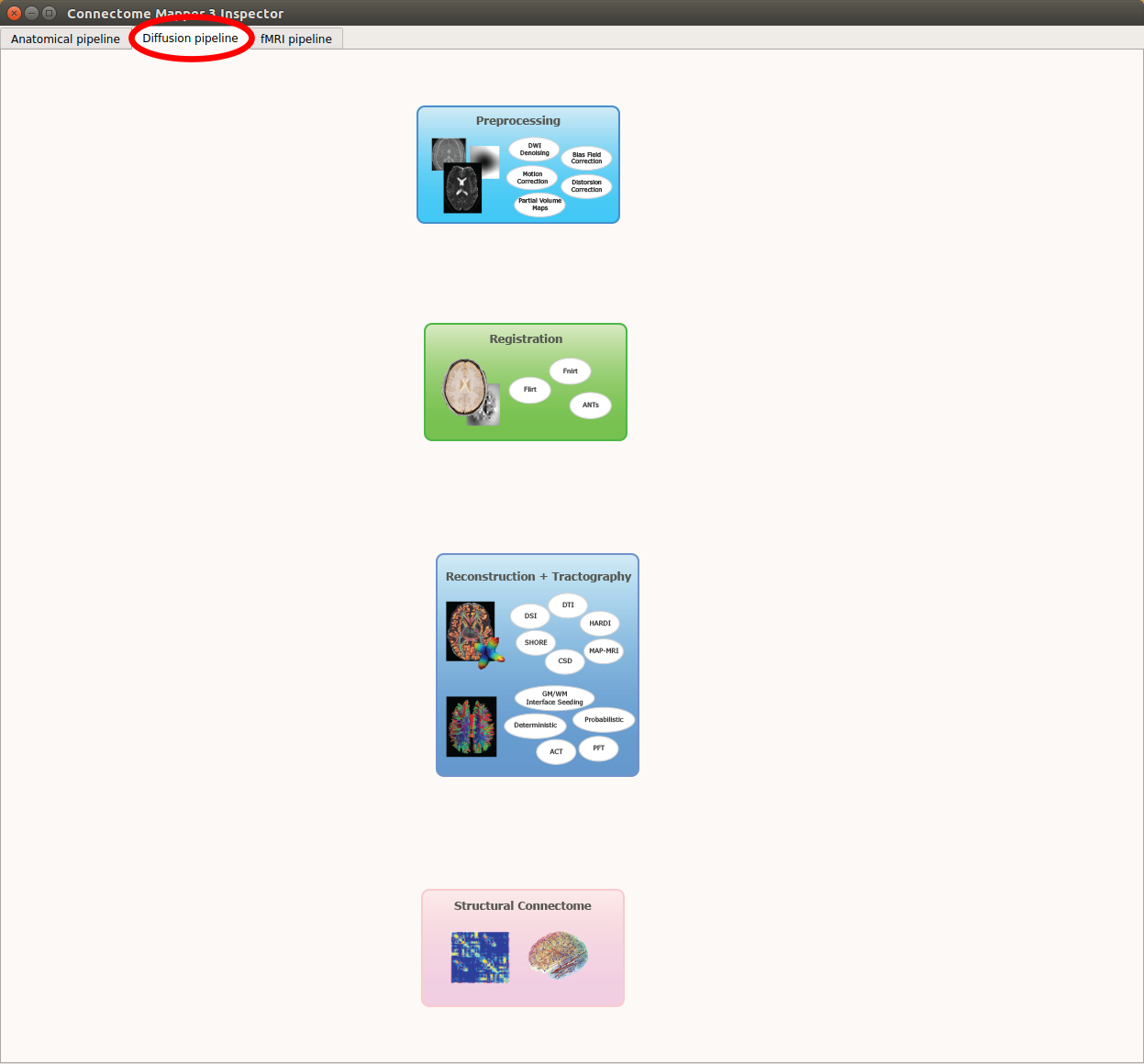
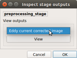
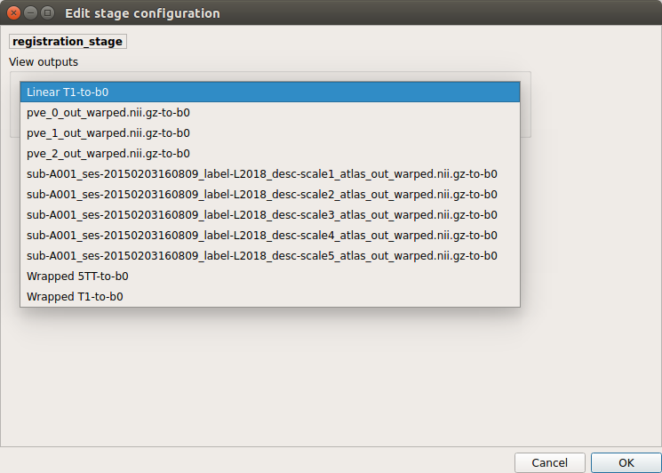
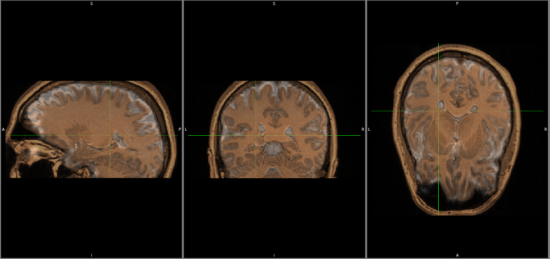
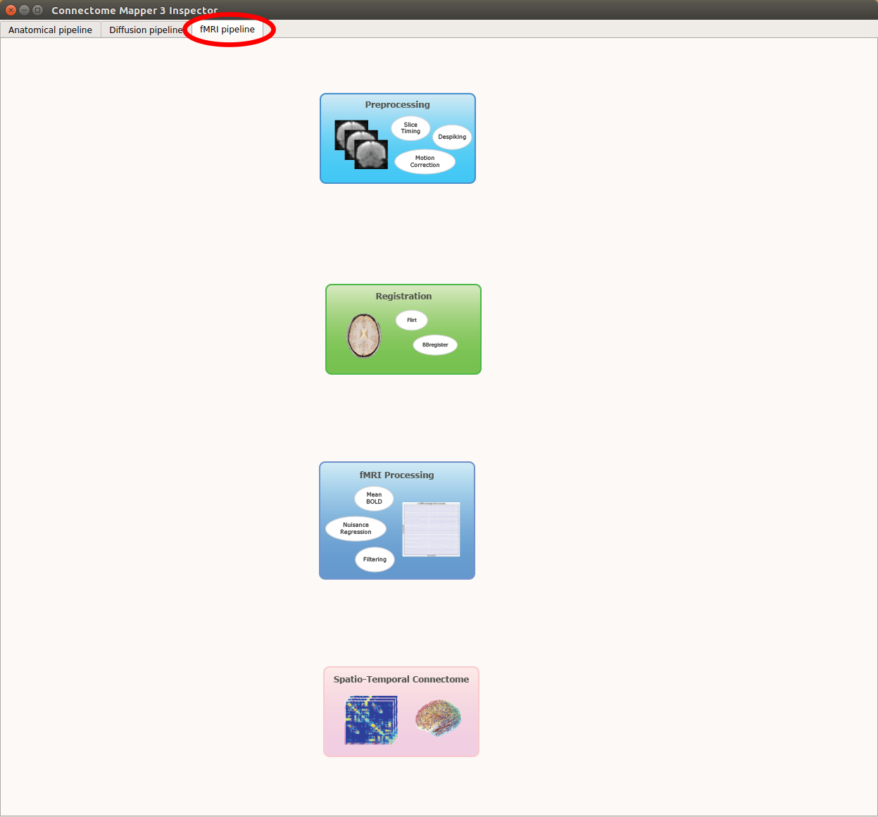
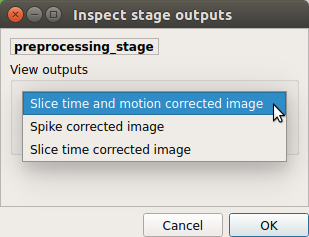
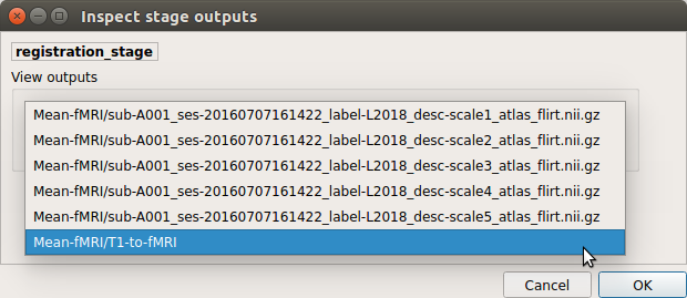
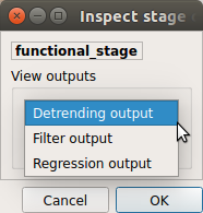
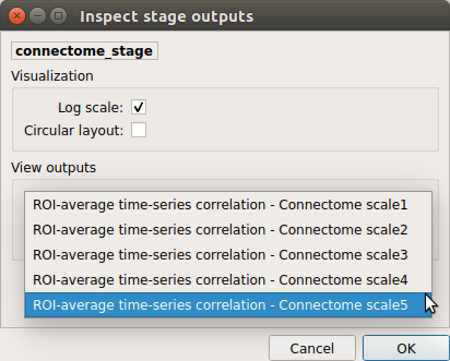
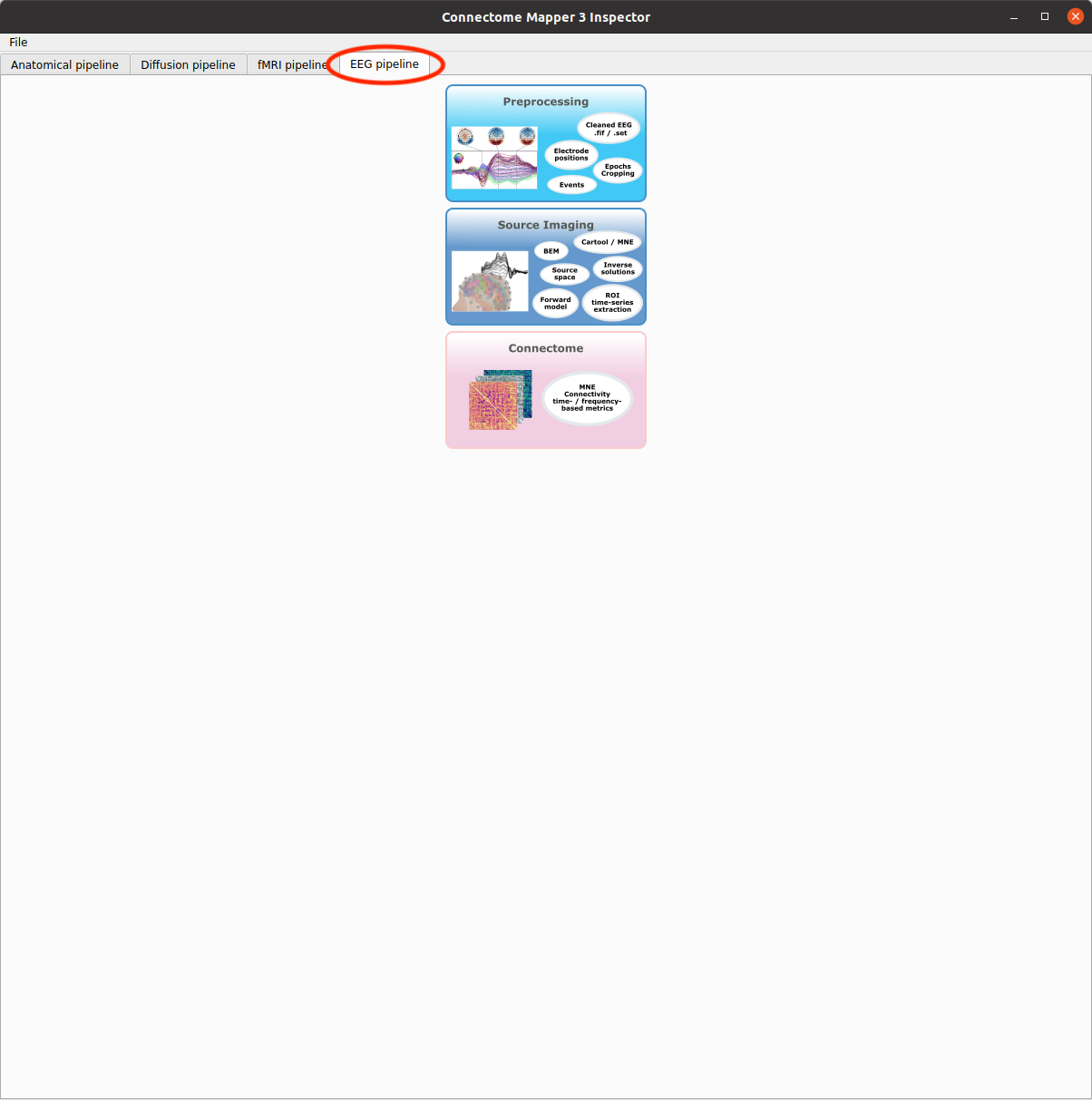
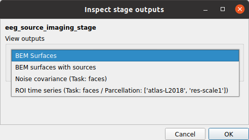
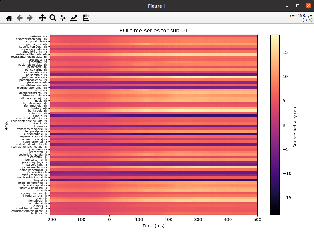
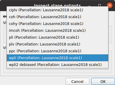
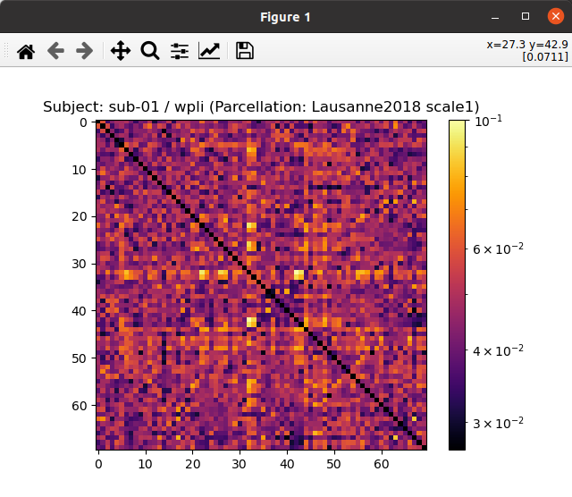
From the main window, click on the right button to start the Inspector Window.
The Connectome Mapper 3 Inspector Window will appear, which will assist you in inspecting outputs of the different pipeline stages (each pipeline has a tab panel).